Time, Clocks, and the Ordering of Events in a Distributed System, Lamport, 1978
In this post, I summarize what I learned from the paper Time, Clocks, and the Ordering of Events in a Distributed System. Lamport published it in Communications of the ACM in 1978. The paper discusses time and clocks in distributed systems in depth. It proposes important concepts and algorithms such as “Happened Before”, logical clock, physical clock, and “State Machine”. It is a classic that every distributed systems reader must read.
1. Problem
Before we start, let’s consider the following problem:
- Someone did something \(A\) and looked at his watch. It read “2020/10/06 13:00”. He claims that \(A\) happened at “2020/10/06 13:00”.
- Another person did something \(B\) and looked at his watch. It read “2020/10/06 13:05”. He claims that \(B\) happened at “2020/10/06 13:05”.
Assume both are honest. Can we say that \(A\) happened before \(B\)? Clearly, we cannot tell which came first, because we don’t know whether their watches are “accurate”. What if the problem changes to the following?
- Someone did something \(A\) and looked at his watch. It read “2020/10/06 13:00”. He claims that \(A\) happened at “2020/10/06 13:00”.
- He made a phone call to another person.
- After the call, the second person did something \(B\) and looked at his watch. It read “2020/10/06 12:55”. He claims that \(B\) happened at “2020/10/06 12:55”.
We can see that clock readings and timestamps cannot describe the order of events accurately. Yet in a distributed system, the order of events often plays a “key role” in many algorithms. So how do we describe this order accurately, or design our clocks to avoid the problem in the example above?
2. What is time
The concept of time is fundamental to our way of thinking. It is derived from the more basic concept of the order in which events occur.
The definition of time is essential for understanding “the order of events” and “concurrency” in distributed systems. Lamport points out that time is derived from a more basic concept: the order in which events occur. For example, when we say something happened at 13:00, we mean it happened after we read 13:00 on the clock and before 13:01. So a clock is a way of discretizing continuous time by “numbering” it.
3. Distributed system
The distributed system in this post consists of several processes that are spatially separated. Events in the same process happen sequentially. Processes communicate by sending and receiving messages. A process can be an independent computer, an independent operating system process, or an independent hardware module inside one computer. From here on, I call a process a “node”. In particular, the communication delay between nodes is not negligible compared with the frequency of events inside a single node.
4. Happened Before: a partial ordering
For events in a distributed system, we define the “happened before” relation, written as “\(\rightarrow\)”. It satisfies the following three conditions.
- (1) If \(a\) and \(b\) are two events on the same node, and \(a\) happens before \(b\), then \(a \rightarrow b\) .
- (2) If event \(a\) is a node sending a message, and \(b\) is another node receiving this message, then \(a \rightarrow b\) .
- (3) If \(a \rightarrow b\) and \(b \rightarrow c\) , then \(a \rightarrow c\) .
Two events are concurrent if and only if \(a \nrightarrow b, b \nrightarrow a\).
We also require \(\rightarrow\) to be irreflexive, that is, \(a \nrightarrow a\) . Clearly, it makes no sense to say that an event happened “before” itself.
To describe this relation intuitively, Lamport introduces the “space-time diagram” shown below. In the diagram, time runs upward along the vertical direction, and the horizontal direction shows different nodes in space. The black dots are events. The wavy arrows are messages.
Recall the “happened before” relation above. We can easily find event pairs in the diagram that satisfy it. For example, \(p_1 \rightarrow r_4\), which is derived from \(p_1 \rightarrow q_2 \rightarrow q_4 \rightarrow r_3 \rightarrow r_4\).
The diagram also has concurrent events, such as \(p_3\) and \(q_3\). In the diagram, we can see that \(p_3\) happens later than \(q_3\) in physical time. But the nodes in the system do not know which one came first.
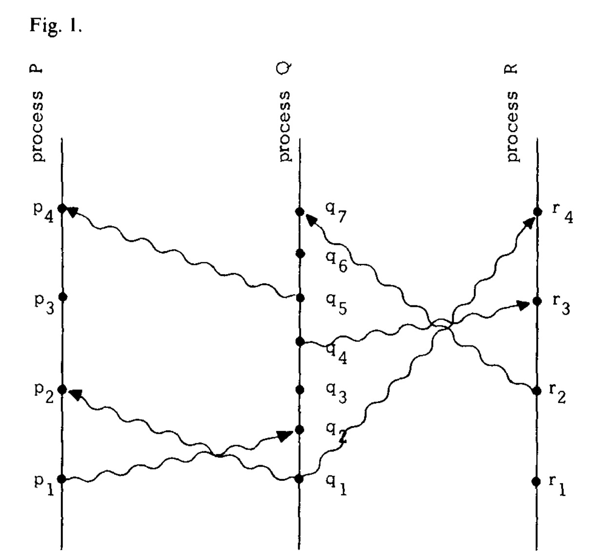 Figure 1. space-time diagram
5. Logical clock
a clock is just a way of assigning a number to an event.
A clock is just a way of assigning a number to an event. More precisely, for each node \(P_i\), we define a clock \(C_i\) as a function. It assigns the number \(C_i \langle a \rangle\) to any event \(a\). For the whole system, the time of any event \(b\) is \(C \langle b \rangle\). If \(b\) happens on node \(P_j\), then \(C \langle b \rangle = C_j \langle b \rangle\). Here we treat the clock as a logical clock inside the system, not a physical clock. Its labels and counting method do not need to agree with physical time. To satisfy the “happened before” partial ordering above, our logical clock must satisfy the following Clock Condition.
Clock Condition. For any events \(a, b\) in the system: if \(a \rightarrow b\), then \(C \langle a \rangle < C \langle b \rangle\).
- C1. If \(a\) and \(b\) are two events on the same node \(P_i\), and \(a\) happens before \(b\), then \(C_i \langle a \rangle < C_i \langle b \rangle\).
- C2. If event \(a\) is node \(P_i\) sending a message, and \(b\) is node \(P_j\) receiving this message, then \(C_i \langle a \rangle < C_j \langle b \rangle\).
In particular, the converse of the Clock Condition, “if \(C \langle a \rangle < C \langle b \rangle\), then \(a \rightarrow b\)”, does not hold. It would require concurrent events to have the same logical time. For example, in Figure 1, both \(p_2\) and \(p_3\) are concurrent with \(q_3\). But by C1, \(C \langle p_2 \rangle < C \langle p_3 \rangle\). So we must have \(C \langle q_3 \rangle \neq C \langle p_2 \rangle\) or \(C \langle q_3 \rangle \neq C \langle p_3 \rangle\). This contradicts the concurrent relation.
For a logical clock, we can imagine “tick” events constantly happening inside a single node. For example, take two consecutive events \(a, b\) on the same node \(P_i\), with \(C_i \langle a \rangle = 4, C_i \langle b \rangle = 7\). Then tick events numbered \(5,6,7\) happen between them. So we can add “tick lines” to the space-time diagram, as the dashed lines in the figure below. By C1, there must be at least one tick line between two consecutive events on the same node. By C2, every message must cross at least one tick line.
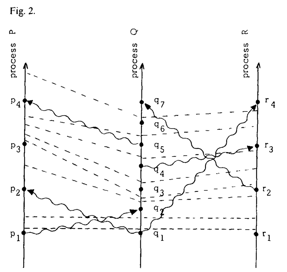 Figure 2
To make this easier to understand, we can redraw the tick lines as equivalent horizontal lines, while keeping the partial ordering of events and messages, as in the figure below.
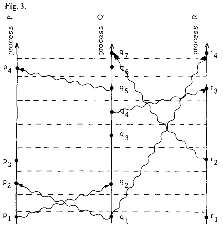 Figure 3
For the logical clock algorithm on a single node, we have the following Implementation Rules.
- IR1. Each node \(P_i\) increments \(C_i\) between any two consecutive events.
- IR2. (a) If event \(a\) is node \(P_i\) sending message \(m\), then \(m\) contains a timestamp \(T_m=C_i \langle a \rangle\). (b) When it receives message \(m\), process \(P_j\) sets its current time \(C_j\) to \(C_j'\), such that \(C_j' \geq C_j\) and \(C_j' > T_m\) .
In practice, when we receive a message, we should run IR2 to update the time first. Then we run the actual event. This guarantees the Clock Condition.
6. Total ordering
With the logical clock, we can sort all events in the system into a total ordering. We first sort events by their time. For events with the same time, we use a priority \(\prec\) predefined on all nodes. The priority can be any rule, such as sorting by id.
More precisely, we define the total ordering \(\Rightarrow\). For event \(a\) on node \(P_i\) and event \(b\) on node \(P_j\), \(a \Rightarrow b\) if and only if (i) \(C_i \langle a \rangle < C_j \langle b \rangle\) or (ii) \(C_i \langle a \rangle = C_j \langle b \rangle\) and \(P_i \prec P_j\).
By the Clock Condition, anything that satisfies the partial ordering \(\rightarrow\) also satisfies the total ordering \(\Rightarrow\).
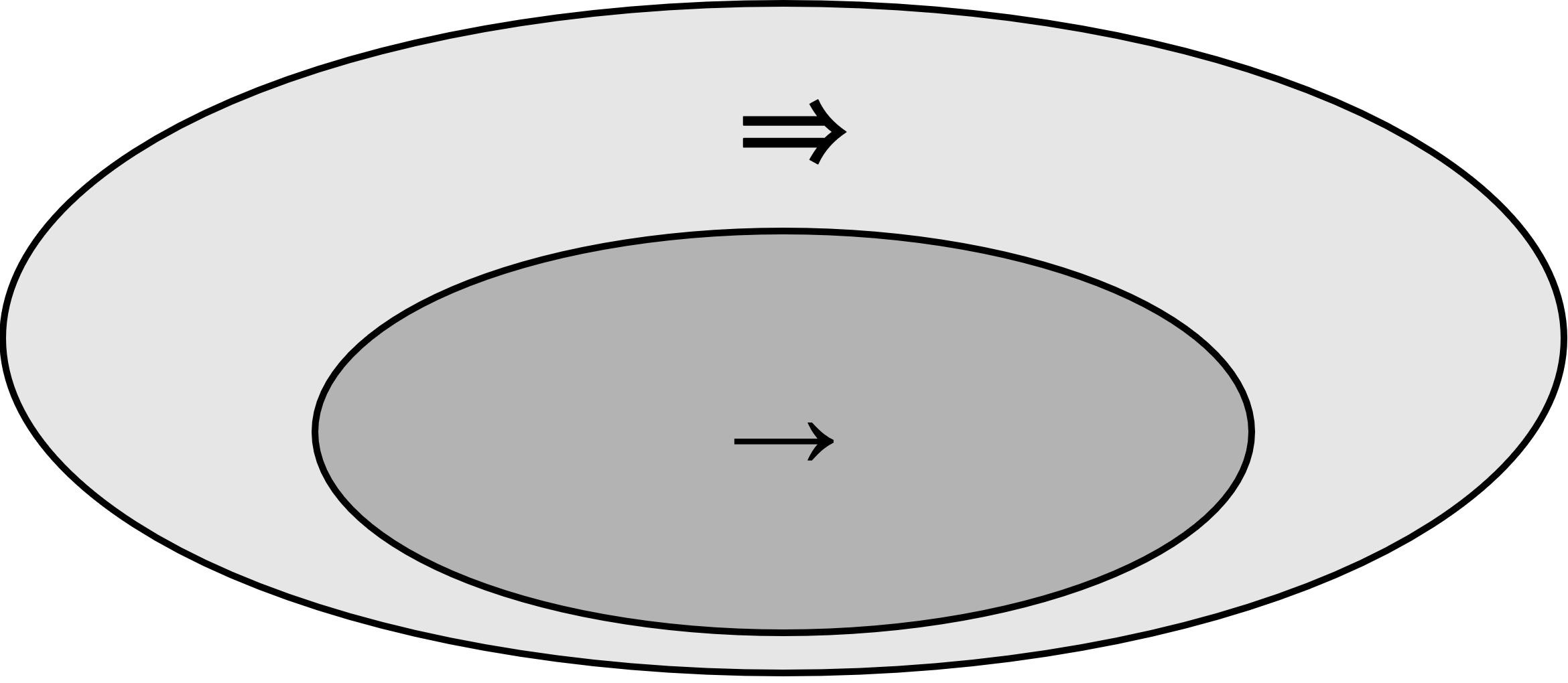 Figure 4. partial ordering and total ordering
7. Physical clock
7.1 Outside the system
Under the total ordering, events outside the system sometimes cause abnormal behavior.
Consider this case. Someone triggers event A on node A, then calls another person. After the call, that person triggers event B on node B. The system knows nothing about the outside event “phone call”. So it is possible to get \(B \Rightarrow A\).
We define the set of all events in the system as \(\varphi\). The set of system events together with external events is \(\underline{\varphi}\). \(\underline{\rightarrow}\) is the happened before relation on \(\underline{\varphi}\). In the example above, we have \(A \underline{\rightarrow} B\), but \(A \nrightarrow B\).
Clearly, no algorithm can guarantee the \(\underline{\rightarrow}\) relation from \(\varphi\) alone, without outside information. To ensure \(A \rightarrow B\), we have two options.
- Introduce the outside information explicitly. For example, event \(A\) happens at logical time \(T_A\). After the call, we tell the system explicitly that the time of \(B\) must be greater than \(T_A\).
- Build a system that satisfies the following Strong Clock Condition.
Strong Clock Condition. For any events \(a, b\) in \(\varphi\): if \(a \underline{\rightarrow} b\) then \(C \langle a \rangle < C \langle b \rangle\).
Clearly, compared with option 1, the Strong Clock Condition is the option we want. Next, I explain how to implement a physical clock that satisfies the Strong Clock Condition.
7.2 Physical clock implementation
Let \(C_i(t)\) be the reading of clock \(C_i\) at physical time \(t\). For mathematical convenience, we assume \(C_i\) is continuously differentiable in \(t\). \(dC_i(t)/dt\) is the rate at which the clock runs at time \(t\).
For \(C_i\) to run at a rate close to real physical time, we need \(dC_i(t)/dt \approx 1\) for all \(t\). More precisely, we need the following condition.
- PC1. There exists a constant \(\kappa \ll 1\) such that for all \(i\) : \(\vert dC_i(t)/dt - 1 \vert < \kappa\). For typical crystal controlled clocks, \(\kappa \leq 10^{-6}\).
Besides keeping each clock accurate, the clocks must also stay synchronized with each other. That is, \(C_i(t) \approx C_j(t)\) for all \(i,j,t\).
- PC2. For all \(i, j\): \(\vert C_i(t) - C_j(t)\vert < \epsilon\). Intuitively, the height difference of a single tick line in Figure 2 cannot be too large.
For PC2, because of accumulated error, two clocks that run completely independently will drift further and further apart. So we need an algorithm to synchronize the clocks on different nodes.
First, we assume our clocks satisfy the Clock Condition. Then we only need to consider the case \(a \nrightarrow b\) in \(\underline{\varphi}\). It is easy to see that \(a\) and \(b\) must happen on different nodes.
Let \(\mu\) be smaller than the minimum communication delay between nodes. That is, event \(a\) happens at physical time \(t\), and event \(b\) happens on another node. If \(a\underline{\rightarrow} b\), then \(b\) happens at \(t + \mu\) at the earliest. Usually, we can set \(\mu\) to the minimum distance between nodes divided by the speed of light.
To avoid the abnormal case above, we must make sure that \(C_i(t + \mu) - C_j(t) > 0\) for any \(i, j\) and \(t\) .
Combining with PC1, we have \(C_i(t + \mu) - C_i(t) > (1- \kappa)\mu\). See Appendix 8.2 for the derivation.
Combining with PC2, we need \(-\epsilon \geq -\mu(1 - \kappa)\), so we need \(\epsilon/(1 - \kappa) \leq \mu\). See Appendix 8.3 for the derivation.
7.2.1 Physical clock algorithm
Next, I describe the algorithm that makes the formulas above, PC1 and PC2 hold.
For a message \(m\) sent at physical time \(t\) and received at physical time \(t'\), we define the total delay of the message as \(v_m = t' - t\). The receiving node does not know the value of \(v_m\). But it can know the minimum delay of the message \(\mu_m\), where \(\mu_m \geq 0\) and \(\mu_m \leq v_m\). We call \(\xi_m = v_m - \mu_m\) the unpredictable delay.
For the physical clock algorithm on a single node, we have the following Implementation Rules.
- IR1’. If node \(P_i\) receives no message at physical time \(t\), then \(C_i\) is differentiable at \(t\), and \(dC_i(t)/dt > 0\).
- IR2’. (a) If \(P_i\) sends message \(m\) at physical time \(t\), then \(m\) contains a timestamp \(T_m=C_i(t)\). (b) When it receives message \(m\) at physical time \(t'\), process \(P_j\) sets its current time to \(C_j(t') = \max(C_j(t' - 0), T_m + \mu_m)\). Here \(C_j(t' - 0) = \underset{\delta \rightarrow 0}{\lim}C_j(t'-\vert \delta\vert )\).
7.2.2 Proof of the physical clock algorithm
Now we prove that the implementation rules above ensure PC2.
We view the whole system as a directed graph. The vertices are the nodes. A directed edge from \(P_i\) to \(P_j\) is a message link.
Let \(d\) be the diameter of the directed graph (longest shortest path). Let \(\tau\) be the minimum communication interval between two nodes. That is, between any time \(t\) and \(t + \tau\), \(P_i\) sends at least one message to \(P_j\). The theorem below tells us how long after system start-up the system reaches a time synchronization that satisfies PC2.
Theorem: Assume the system is a strongly connected graph with diameter \(d\) that follows IR1’ and IR2’. For any message \(m\), \(\mu_m \leq \mu\), where \(\mu\) is a specific constant, for all \(t \geq t_0\). (a) PC1 always holds. (b) There are constants \(\tau\) and \(\xi\) such that, on every edge of the system, a message with an unpredictable delay of at most \(\xi\) is sent every \(\tau\) seconds. Then PC2 is satisfied for all \(t\gtrapprox t_0 + \tau d\), with \(\epsilon \approx d(2\kappa\tau + \xi)\) and \(\mu + \xi \ll \tau\). The proof is in Appendix 8.4.
8. Appendix
8.1 Total Ordering Application: Mutual Exclusion Problem
8.2 Derivation of PC1
By PC1, \(\left \vert \frac{C_i(t+\mu) - C_i(t)}{\mu} < \kappa \right \vert\). So \((1 - \kappa)\mu < C_i(t+\mu) - C_i(t) < (1 + \kappa)\mu\) .
8.3 Derivation of PC2
Continuing from 8.2, \(C_i(t) + \mu(1-\kappa) < C_i(t+\mu)\).
So for \(C_i(t + \mu) - C_j(t) > 0\), we need \(C_i(t) - C_j(t) > -\mu(1 - \kappa)\).
By PC2, \(C_i(t) - C_j(t) < -\epsilon\).
So we get \(\epsilon \leq \mu(1 - \kappa)\).
8.4 Proof of the theorem
For any \(i\) and \(t\), we define \(C_i^t\) as a clock that is set to \(C_i\) at time \(t\), runs at the same rate as \(C_i\), and is never reset. That is,
\[C_i^t = C_i(t) + \int_{t}^{t'}[dC_i(t)/dt]dt \tag{1}\]For all \(t' \geq t\), because \(C_i\) can be reset, we note that
\[C_i(t') \geq C_i^t(t') \tag{2}\]Suppose \(P_1\) sends a message to \(P_2\) at time \(t_1\). \(P_2\) receives it at time \(t_2\). The unpredictable delay is \(\leq \xi\), and \(t_0 \leq t_1 \leq t_2\). Then for all \(t \geq t_2\), we have
\[\begin{aligned} & C_2^{t_2}(t) \geq C_2^{t_2}(t_2) + (1 - \kappa)(t - t_2) & \qquad [by\ (1)\ and\ PC1] \\ & \geq C_1(t_1) + \mu_m + (1 - \kappa)(t - t_2) & \qquad [by\ IR2'(b)] \\ & = C_1(t_1) + (1 - \kappa)(t - t_1) - [(t_2 - t_1) - \mu_m] + \kappa(t_2 - t_1) \\ & \geq C_1(t_1) + (1 - \kappa)(t - t_1) - \xi \end{aligned}\]So, using these assumptions, for all \(t \geq t_2\) we get
\[C_2^{t_2}(t) \geq C_1(t_1) + (1 - \kappa)(t - t_1) - \xi \tag{3}\]Now suppose that for \(i =1,...,n\), we have \(t_i \leq t_i' < t_{i+1}, t_0 \leq t_1\). At \(t_i'\), \(P_i\) sends a message to \(P_{i+1}\). The message is received at \(t_{i+1}\), and its unpredictable delay is less than \(\xi\). Applying equation (3) repeatedly, for \(t \geq t_{n+1}\) we get
\[C_{n+1}^{t_{n+1}}(t) \geq C_1(t_1') + (1 - \kappa)(t - t_1') - n\xi \tag{4}\]From PC1, IR1’, and IR2’, we can derive
\[C_1(t_1') \geq C_1(t_1) + (1 - \kappa)(t_1' - t_1)\]Combining this with (4) and (2), for \(t \geq t_{n+1}\) we get
\[C_{n+1}(t) \geq C_1(t_1) + (1 - \kappa)(t - t_1) - n\xi \tag{5}\]For any two nodes \(P\) and \(P'\), we can find a sequence of nodes \(P = P_0, P_1, ..., P_{n+1} = P', n \leq d\). By assumption (b), we can find times \(t_i, t_i'\) such that \(t_i' - t_i \leq \tau\) and \(t_{i+1} - t_i' \leq v\), where \(v=\mu + \xi\). So inequality (5) holds for any \(t \geq t_1 + d(\tau + v)\), with \(n \leq d\). For any \(i, j, t, t_1\) with \(t_1 \geq t_0\) and \(t \geq t_1 + d(\tau + v)\), we therefore have
\[C_i(t) \geq C_j(t_1) + (1 - \kappa)(t - t_1) - d\xi \tag{6}\]